Voxel Debut
Posted Aug. 17, 2016 by Francesca SargentRecently, we were approached by Dr Karen Anderson of the University of Exeter to visualise voxel data of Bedford, Luton and Milton Keynes.
A natural place to start with the data would have been to interpret it in Python and recreate the cities in Minecraft, so of course I became distracted and found myself being led down a different, more Fluxus/3D/performative inspired path. However, the first port of call was to actually read the data, which requires a brief explanation of the data format.
Dr Stefano Casalegno kindly donated us full-waveform lidar data of the greenspace of Milton Keynes. I guess firstly, I should note that in computing, a voxel can be considered as a volumetric pixel, representing a three dimensional unit, as opposed to a pixel’s two dimensional unit. The city was scanned by a laser/sensor in 390sq meter areas – each ’tile’ is saved as a GeoTIFF, comprising of ~67000 1.5m x 1.5m x 0.5m voxels representing the density of the objects within that space as read by the laser. Density values range from 1, being dense & impenetrable, to -1, being nothing. Values in between can represent semi-translucent leaves and the like.
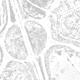
Opening the GeoTIFF in previewing software, predictably, displays the image as an aerial photograph of the area.
Furthermore, for each x and y coordinate of the tile, there are 70 ‘heights’ of which the tile data was taken, starting at 0 and incrementing by 0.5m each time. Thus, there are 70 GeoTIFF images per 260sqm of Milton Keynes. When each GeoTIFF ’tile’ is stacked, it becomes a three dimensional representation of the space. And a lot of data to play with!
Python’s Imaging Library (PIL) served as a really useful library for reading the GeoTIFF data. I reigned in a collection of images from one x,y coordinate, upto 70 on the z coordinate. Plainly, images of all 70 height levels of one particular area, starting from the ground to the sky. Opening the image returned arrays of integers between -1 and 1, as predicted, but interestingly some ‘nan’ too – this will be followed up, but for now 0 would suffice in place.
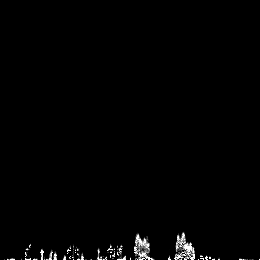
While looking at all of the values was great fun, Dave had the magnificent idea to stack the images and create cross sections of the area, changing the perspective from aerial to frontal view. This required creating 260 images, cross referencing the 70 existing images and using the index of that image to copy a line from the nth y-pixel of that image, rendering the values as a greyscale value (0 – 255) per pixel, and saving each out as a png. The result? When viewed in sequence, a walkthrough of that small area.
Here’s a gif of the result!
This is exciting, because firstly, we have a lightweight tool for handling the data and outputting images. Secondly, it means that this data can be can be interpreted in many ways, independent of GIS software – leading to the daydreaming of other possible outputs with confidence, such as 3D Printing or rendering as a 3D object. The fact that we can isolate the greenspace away from buildings, also, leads to interesting ideas of representation (3D printing moss?!). Soon, I will rebuild Milton Keynes (at least parts of it) in Minecraft, however with a couple of Algoraves coming up this week, it made sense to incorporate the voxels into Fluxus. This requires a new post, however, as the subject matter is changing….
The project itself can be found on Github
Created: 15 Jul 2021 / Updated: 15 Jul 2021


